class: center, middle, inverse, title-slide # G-estimation of structural nested models ## What If: Chapter 14 ### Elena Dudukina ### 2021-11-10 --- # 14.1 The causal question revisited - generalized methods for treatment contrasts that vary over time - models whose parameters are estimated via g-estimation are structural nested models - each g-method has a different set of modeling assumptions --- # 14.1 The causal question revisited - Total effect and no censoring: `\(E[Y^{a=1, c=0}]\)` - `\(E[Y^{a=0, c=0}]\)` - Effect in the stratum: `\(E[Y^{a=1, c=0}|sex=1]\)` - `\(E[Y^{a=0, c=0}|sex=1]\)` - IPT-weighted MSM with interaction term - Standardisation in the stratum of interest - g-estimation --- # 14.1 The causal question revisited - g-estimation to estimate the average causal effect of smoking cessation A on weight gain Y in each strata defined by the covariates L - `\(E[Y^{a=1, c=0}|L]\)` - `\(E[Y^{a=0, c=0}|L]\)` --- # 14.2 Exchangeability revisited - Conditional exchangeability: the outcome distribution in the treated and the untreated would be the same if both groups had received the same treatment level: `\(Y^a \perp\perp A|L\)` for `\(a=0\)` and `\(a=1\)` - Knowing the value of `\(Y^{a=0}\)` does not provide information (help distinguish) between exposure levels: `\(Pr[A=1|Y^{a=0}, L]\)` = `\(Pr[A=1|L]\)` - `\(logitPr[A=1|Y^{a=0}, L] = \alpha_0 + \alpha_1Y^{a=0} + \alpha_2L\)` and so `\(\alpha_1=0\)` --- # 14.3 Structural nested mean models - Assuming no censoring: `\(E[Y^{a=1}|L]\)` - `\(E[Y^{a=0}|L]\)` - Structural model for the conditional causal effect: `\(E[Y^{a=1} - Y^{a=0}|L]\)` = `\(\beta_1*a\)` - Structural model for the conditional causal effect with EMM by L: `\(E[Y^{a=1} - Y^{a=0}|L]\)` = `\(\beta_1*a + \beta_2*a*L\)` - under conditional exchangeability: `\(E[Y^{a=1} - Y^{a=0}|L, A=a]\)` = `\(\beta_1*a + \beta_2*a*L\)` (**structural nested mean model**) - `\(\beta_1\)` and `\(\beta_2\)` are estimated using g-estimation - Nested model means it is "nested" when the treatment is time-varying --- # 14.3 Structural nested mean models - Structural nested models are semiparametric - Agnostic about the intercept and the effect of L t(no parameter `\(\beta_0\)` and no parameter `\(\beta_3\)`) - Fewer assumptions and potentially more robust to model misspecification than g-computation of the parametric g-formula --- # 14.3 Structural nested mean models - Assuming censoring: `\(E[Y^{a=1, c=0}|L]\)` - `\(E[Y^{a=0, c=0}|L]\)` - G-estimation can be used to adjust for confounding but not selection bias - Need IP weighting for selection bias, first - Nonstabilized IP weights for construction of pseudo-population: - $W^C = 1/pr[C=0|L, A - In pseudo-population without censoring: * `\(E[Y^{a=1, c=0}|L, A]\)` - `\(E[Y^{a=0, c=0}|L, A]\)` * = `\(E[Y^{a=1, c=0} - Y^{a=0, c=0}|L, A]\)` * = `\(\beta_1*a + \beta_2*a*L\)` --- # 14.4 Rank preservation - Rank each subject according to their observed `Y` - Rank according to subjects' counterfactual outcomes `\(Y^a\)` - 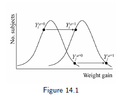Had both lists `\(Y^{a=0}\)` and `\(Y^{a=1}\)` were in the same, there was rank preservation - Treatment has no effect on no one's outcome (sharp null hypothesis), the rank preservation holds - The conditional rank preservation holds when effect of `A` on `Y` is the same - Rank preserving structural model: `\(Y^{a=1}_i - Y^{a=1}_i = \psi_1a + \psi_2a * a*L_i\)` with `\(\psi_1 + \psi_2*l\)` is the causal effect for all individuals `\(i\)` with `\(L=l\)`  - However, the outcomes nearly never are expected to be constant on an individual level and so (additive) rank preservation is implausible. - Average causal effects are agnostic about the the individual causal effects. - Never use rank preservation model in practice, however, it is used in the section 14.5 --- # 14.5 G-estimation - Estimate parameters of the structural nested mean model: `\(E[Y^{a=1} - Y^{a=0}|L, A=a]\)` = `\(\beta_1*a\)` - No `\(\beta_2*a*L\)` term assumes constant treatment effect across strata of `\(L\)` (no additive effect measure modification (EMM) by `\(L\)`) - Additive rank preservation model assumes that effect of `\(A\)` is constant and the same for all individuals and average causal effect `\(\beta_1\)` is the same as `\(\psi_1\)` individual causal effect (although implausible in real life) - Rank preserving model `\(Y^{a=1}_i - Y^{a=0}_i = \psi_1a\)` or `\(Y^{a=0} = Y^{a=1}_i - \psi_1a\)` --- # 14.5 G-estimation - 1st step: linking the model and the observed data - By consistency: `\(Y^{a=1} = Y\)` among `\(A=1\)` and `\(Y^{a=0} = Y\)` among `\(A=0\)` - Under rank preservation and correctly specified model: `\(Y^{a=0} = Y^{a=1}_i - \psi_1a\)` is `\(Y^{a=0} = Y - \psi_1A\)` - `\(\psi_1\)` is unknown and the aim of the analysis is to estimate `\(\psi_1\)` - To compute `\(\psi_1\)` make guesses: 1) -20 2) 0 3) 10 - Then compute: `\(H(\psi^*) = Y - \psi^*A\)` - If conditional exchangeability holds: `\(\alpha_1 = 0\)` in the logistic regression model for treatment: - `\(logitPr[A=1|H(\psi^*), L] = \alpha_0 +\alpha_1H\psi^* + \alpha_2*L\)` - The guess that gets us closer to `\(\alpha_1 = 0\)` is the most correct guess - 95% CI for `\(\psi^*\)` is computed based on a set of guesses that are tested against the H0 and results with P-values > 0.05 are the limits that form 95% CI --- # 14.6 Structural nested models with two or more parameters - In the presence of the EMM, the model in the previous slides was misspecified and the answer given was incorrect - The EMM by `\(V\)` requires estimation of the term `\(\beta *a*V\)`: `\(E[Y^{a=1} - Y^{a=0}|L, A=a]\)` = `\(\beta_1*a + \beta *a*V\)` corresponding to the rank preserving model `\(Y^{a=1}_i - Y^{a=0}_i = \psi_1a + \psi_2*a*V_i\)` - The logistic model for treatment them will be: `\(logitPr[A=1|H(\psi^*, L) = \alpha_0 + \alpha_1 H(\psi^*) + \alpha_2H(\psi^*)V + \alpha_3 L]\)`, where `\(H(\psi^*)=(\psi^*_1, \psi^*_2)\)` - The values of `\(\psi^*_1\)` and `\(\psi^*_2\)` produce `\(H0(\psi^*) \perp\perp A |L\)`, or we need to find guesses that result in `\(\alpha_1\)` and `\(\alpha_2\)` both being zero. --- # References 1. Hernán MA, Robins JM (2020). Causal Inference: What If. Boca Raton: Chapman & Hall/CRC (v. 30mar21) 2. https://remlapmot.github.io/cibookex-r/g-estimation-of-structural-nested-models.html